
Learning Probabilistic State Machines using FlexFringe
Sicco Verwer ·Probabilistic Deterministic Automata
A PDFA is a generative model for discrete sequences. Starting from the root node, it follows transitions, outputting the symbol associated with each transition in sequence. For instance, in the below figure, following the transition labeled by “a” from the root changes the current state (the root, a rectangle, indicated by the arrow from I) to state 1. The numbers at each transition denotes the count of that transition in the data used to train the model. In each state, a number is written, followed by the number of total occurrences (after the #, larger states have a higher count). We normalise the transition counts to obtain transition probabilities, e.g., the probability of an “a” transition from the root is 6/(6+7) = 0.46 (the counts of the transition divided by the sum of all outgoing transition counts). The probability of a sequence is the product of the probabilities of the transitions. Thus sequence “abbab” has (approximate) probability 0.46*0.67*1.0*0.46*0.67 = 0.09.
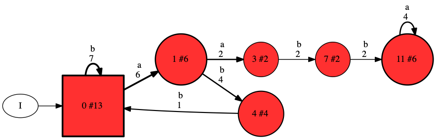
Optionally, Flexfringe can add the final probability (stopping chance, option —finalprob=1). For this it uses the state counts, which include the traces ending in the states. This probability for state 4, in which “abbab” ends is 3/4 since 4 sequences reach state 4, but there is only 1 count on outgoing transitions, leaving 3 ending sequences. Using these would give probability 0.09*0.75 = for “abbab”. Theoretically, these two options model different kinds of sequence distributions. Whether to use final probabilities in practice build down to deciding whether the ending of a sequence hold information or not. For instance, when using sliding windows to collect data, it does not as the stopping point is determined by us, not by the system.
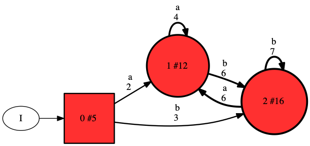
The model in the above figure is both probabilistic and deterministic. As this may be confusing, I will explain what this means. The model is clearly probabilistic as it represents a probability distribution that may be used to generate sequences. Like any probabilistic model, we may use this distribution to detect outliers or anomalies, compute distances between models, and detect similarities. The model is also deterministic because (unlike for instance hidden Markov models), the model follows a unique path for each possible sequence. More specifically, given a current state (e.g., the root), a next symbol (e.g., “a”), there is only one possible next state (e.g., 1). Although it is deterministic, the model is much more powerful than a Markov chain, which on the same data gives the model depicted below (obtain using option —markovian=1).
Learning
The states in the above models are red. The reason is that FlexFringe implements the so-called red-blue framework. It maintains a core of red states with a fringe of blue states, the remaining states are white. The red states denote the part of the PDFA that has already been learned. FlexFringe greedily and iteratively tries to merge blue states with red ones, identifying a new transition (such as a loop). FlexFringe contains a multitude of heuristics and consistency checks that respectively govern the score of a merge and whether it can be merged at all. FlexFringe always performs the highest scoring consistent merge. When a blue state cannot be merged with any red (all checks are inconsistent), it is colored red and its children blue. There are several possible priority orders that can be used to decide which blue state to consider next. Typically, we let FlexFringe consider only the blue state with highest state count (parameter —largestblue=1), i.e., the one that is visited most en thus contains the most information.
The details of the consistency checks are somewhat complex. I try to provide some insight into how they work using a small example FlexFringe run. We provide FlexFringe with the following input file in Abbadingo format (a famous DFA learning competition from 1998):
5 2
1 2 a b
1 5 b b b a b
1 6 b a a b b a
1 8 b a b b b b a b
1 7 a a b b a a a
The first line is the header, specifying the amount of sequences and the size of the alphabet (number of possible symbols/words). Each line after that contains a sequence. The first symbol/word denotes the sequence type. In this case, all sequences are positive. The number after that denotes the length of the sequence. The sequence if written after that. For example, the first sequence is “a b” and the second is “b b b a b”. FlexFringe parses this file, and creates an initial model called the prefix tree, shown below.
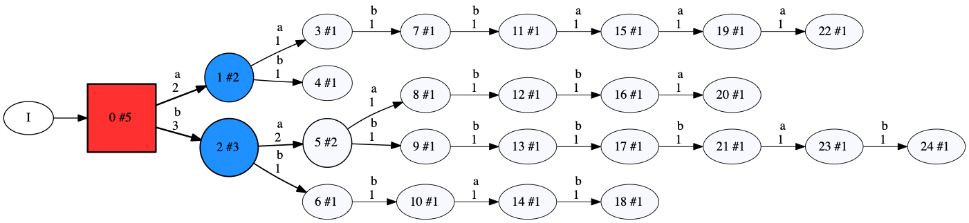
This prefix tree encodes directly the input data. There exists exactly one path for each possible trace and the counts are exactly the occurrence counts from the input data. Initially, only the root state is red and its children are blue. It considers merges between the root and state 2 because this is the most visited blue state. As heuristic we use Akaike’s Information Criterion (AIC), which is a popular and often effective heuristic for learning PDFAs. According to the tests performed by this heuristic, state 1 is consistent with the root, and is therefore merged:
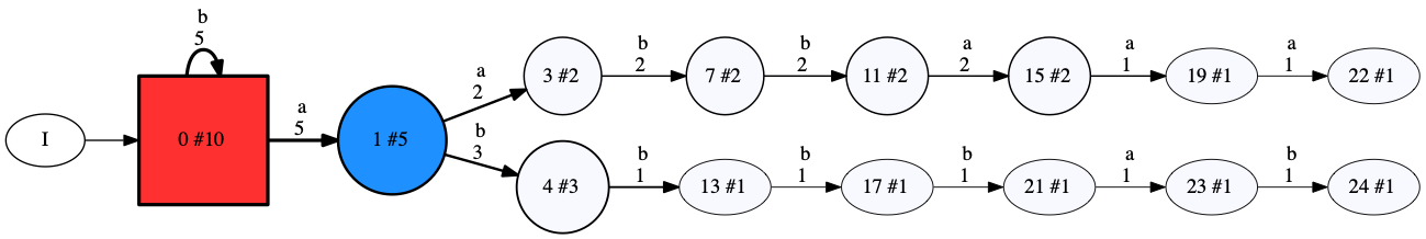
What has happened? Firstly, we see that state 0 (the root) contains a self-loop with label “b”. Any transition to state 2 has been redirected to target state 0. The same happened to all transitions from state 2, which now have state 0 as source state. However, in FlexFringe models are never allowed to be non-deterministic. As state 0 would now have two outgoing transitions with label “a”, one to state 1, and another to state 5 obtained from the merge, the targets of these transitions (states 1 and 5) have to be merged as well. This process, called determinization, is iteratively applied until all non-deterministic transitions are gone. This also explains why the obtained model is much smaller; there is a lot of overlap in sequences that occur after visiting the root state and state 2. It is this overlap (including their frequency) that is measured by the AIC heuristic, and it is deemed sufficiently similar to allow this merge.
At first sight, you may think the state and transition counts are incorrect. Before, state 0 had an outgoing transition with label “b” that occurred 3 times. In the new model it occurs 5 times. The reason for this is simple, the counts include the counts from merges that happened during the determination process. You can check that there are 5 “b” counts in total to states 2, 6, and 10 in the earlier model. Similarly, state 1 now has 2 outgoing “a” transitions and 3 outgoing “b” transitions, obtained from merges with states 5 and 14. Note that these new counts are the ones used in probability calculations. Thus, by merging, the probability that a sequence starts with an “a” event has changed from 2/3 to 5/10. Naturally, it is the job of the heuristic functions and consistency checks to make sure these probabilities do not change too much from the original probabilities in the prefix tree.
The next few steps taken by FlexFringe are all extend actions: it colors the considered blue state red and its children blue. There apparently exists no consistent red-blue merge for these states. In other words, the futures of these states are all considered to be sufficiently different by the consistency check to prevent merging.You can check this yourself by comparing the counts and labels of outgoing transitions of all states that would have been merged during determinization of such a merge. This is exactly what FlexFringe checks as well. The first extend action results in the following model, the model obtained after the last extend action is shown just below it.

Now, FlexFringe does find a consistent merge, learning a self loop with label “a”. This result is depicted below. This is not very surprising since the model above shows a sequence of three outgoing “a” labels without any other behaviour present. What might be more surprising is that such a loop is not identified for the “b” label transitions that occur just before (before state 11). There is a sequence of 2 “b” labels, without other behaviour. A self-loop with a “b” in state 3 seems possible, but this would also have merged states 3 and 11 due to determinization. Clearly, states 3 and 11 are different since 3 only has “b” as outgoing transition label, while state 11 only has outgoing label “a”. The AIC heuristic finds this different sufficient to prevent the merge from happening.
A run of FlexFringe on the HDFS dataset
The HDFS dataset, obtained from the DeepLog work https://github.com/wuyifan18/DeepLog, contains discretised logs from runs of a Hadoop server. The first few lines (modified for FlexFringe input) looks like this:
4855 50
1 19 5 5 5 22 11 9 11 9 11 9 26 26 26 23 23 23 21 21 21
1 13 22 5 5 5 11 9 11 9 11 9 26 26 26
1 21 22 5 5 5 26 26 26 11 9 11 9 11 9 2 3 23 23 23 21 21 21
1 13 22 5 5 5 11 9 11 9 11 9 26 26 26
So the file contains 4855 sequences and an alphabet of size 50 (this is an upper bound, the latest version off FlexFringe does not require this parameter, but reads is as it is still part of the original format). The first sequences has type 1 (all are positive) and length 19. It starts with a block of 5 and 22 events, followed by 11 and 9 events, some 26 events, and ending with 23 and 21 events. Note that although the events are integers, FlexFringe treats all as discrete symbols (it parses each symbol as a string). A run of FlexFringe on this data:
./flexfringe ~/Downloads/hdfs_train.dat –ini=ini/aic.ini
should provide an output to the console similar to (sometimes we update/improve heuristics which can lead to slightly different output):
Using heuristic aic
Creating apta using evaluation class aic
batch mode selected
starting greedy merging
x3595 x2593 x1637 x1637 x1575 x1570 x1471 x1466 x1268 x1268 x1268 x1268 x1268 x1258 x1257 x1257 x1255 x999 x999 m964.25 x1194 x1194 x1194 x1194 x1194 x1194 m1275.92 x864 x794 x668 x663 x657 x657 x653 x651 x651 x467 m645.639 x422 x333 m362.693 x268 m2.68143 x204 x195 m294.762 x191 x190 x181 m249.579 x181 x154 m121.705 x223 x140 x134 x129 x118 x117 m325.296 m46.8638 x202 m11.8678 m11.9182 x106 x106 x103 m254.072 x99 x96 m97.7323 x158 x96 x94 m11.9354 x89 m92.8487 m6.74493 x84 x80 m24.3373 m182.913 m89.8854 m13.8054 x106 m314.409 m572.133 m11.9488 m95.3256 m143.703 m448.317 x52 x51 m11.9698 x45 x42 x42 x42 m6 m127.008 x49 x41 m181.521 x44 m115.915 m97.2368 x33 x32 x31 x31 m148.24 x28 m224.446 x27 m11.9847 x25 x25 x24 x23 m173.029 x23 x23 x22 x22 m32.3296 x21 x19 x18 m47.2007 x18 x18 x18 x18 x16 m29.1345 m60.5069 m66.8282 m65.0012 m35.6827 x13 x13 x13 x13 m14.0242 m3.52817 x11 m32.8987 x20 x12 m68.7307 m86.3202 m70.3322 m4.83536 m11.9892 m75.7609 m85.3586 m11.9946 m25.4395 x9 x9 x9 x9 m31.795 x9 x8 x8 m33.0757 m11.9263 m49.3081 m36.1753 x11 x11 m75.4609 m31.2837 x7 m94.363 m11.9963 m11.9963 x6 m31.4996 m30.2795 x6 x6 x6 x5 x5 x5 m91.7534 m72.9108 x5 m30.4953 x5 m17.1579 m3.26506 m72.7619 x5 x4 m74.3226 m84.0499 x4 m47.7217 m45.5452 m7.31236 x6 x6 x3 x3 x3 x3 m2.06037 x3 x3 x3 x3 m0.515196 x5 m2.50647 x3 x3 m18.6577 m37.676 m2.54274 m3.439 x6 x6 x6 x6 x6 x6 x5 x5 m31.4534 m37.9336 m49.7164 m51.1283 x2 x2 x2 m2.49729 x2 x2 x2 m3.88359 x3 m0.596274 x2 x2 m0.454823 m0.73997 x3 x2 x2 m14.4548 x2 x2 x2 x2 x2 x2 x2 m5.68254 m11.9984 m27.1425 x2 x2 m5.97743 x2 x2 m29.2204 m20.3954 m14.2934 m14.4291 x2 x2 x2 m40.2204 m11.999 x2 m29.8035 m6 m6.84619 x2 x2 m7.8777 x2 m5.22741 m9.22741 m2 m11.999 m37.5598 x2 x2 x1 m27.4491 m8.52849 m28.3602 x1 m20.0123 m20.6622 m17.1205 m16.5799 m2.86193 m10.2512 m12.4599 m11.7458 x1 m2.57877 m10.7118 x1 x1 m19.7585 m2 x1 x1 m20.1478 x1 m7.99949 m6.6482 m3.05381 m16.0269 m23.9067 m13.9995 m14.0545 m2 no more possible merges
deleted merger
The default AIC heuristic uses final probabilities (—finalprob=1) and only considers merging the largest blue state (—largestblue=1), instead of any red-blue combination. This latest setting is a speedup parameter, but also when using statistical tests as a heuristic it makes a lot of sense to start with the states that contain the most information. In the console output FlexFringe prints every merge step applied (mSCORE, where SCORE is the AIC improvement). It also prints extend steps (xNUMBER, where NUMBER is the state occurrence frequency). These are blue states that cannot be merged with any red state, and therefore are coloured red. As output, FlexFringe produces a dot file and a json file. The dot file is for visualisation while the json is use for further processing (such as making predictions). Let us take a look at the produced model:
dot ~/Downloads/hdfs_train.dat.ff.final.dot -Tpng -o hdfs.png
open hdfs.png
should give:
which shows the logs block structure mentioned above in a state machine form. FlexFringe is quite an effective method for finding such blocks and their sequential composition and recursive patterns (loops). The HDFS logs also contain parallel processes, which currently leads to a blowup in the state space. This works fine when the parallel processes are executed sufficiently frequent (such as the 22-5 events at the start). It creates issues with less frequent processes (such as the 11-9-5 path after the initial 5). Making FlexFringe cope better with parallelism is an open research problem.
The states in the model show numbers and the state sizes. All states are red since the process finished. More frequent states are displayed as larger circles. Optionally, you can make FlexFringe output state information that is used in the statistical tests (symbol counts and final counts, —printevaluation=1). To provide some more insight into the learning process, we printed the state machine obtained after every merge during this run (—printeachstep=1), but with printing the white states from the prefix tree, and only printing the red and blue states (set with —printwhite=1, and —printwhite=0, —printblue=1):
The model provides some insight into the inner workings of the software that generated the data. Moreover, since it is a probabilistic model, it (the json output) can be used to make predictions and compute probabilities for anomaly detection:
./flexfringe ~/Downloads/hdfs_test_normal.dat –ini=ini/aic.ini –mode=predict –aptafile=”/Users/sicco/Downloads/hdfs_train.dat.ff.final.json”
Using heuristic aic
Creating apta using evaluation class aic
predict mode selected
reading apta file - /Users/sicco/Downloads/hdfs_train.dat.ff.final.json
deleted merger
which gives a csv file (“;” separated) as output, with first few lines:
head /Users/sicco/Downloads/hdfs_train.dat.ff.final.json.result
row nr; abbadingo trace; state sequence; score sequence; sum scores; mean scores; min score
0; “1 19 5 5 5 22 11 9 11 9 11 9 26 26 26 23 23 23 21 21 21”; [1,4,10,16,22,30,40,54,69,84,94,100,103,107,115,124,133,143,152,152]; [-0.300465,-0.326728,-0.45995,0,-0.0441478,-0.00605185,-0.0842081,-0.00313614,-0.166743,0,0,0,-0.000779525,-0.564968,0,0,-0.000256443,0,0,0]; -1.95743; -0.0978717; -0.564968
1; “1 13 5 5 22 5 11 9 11 9 11 9 26 26 26”; [1,4,11,16,22,30,40,54,69,84,94,100,103,103]; [-0.300465,-0.326728,-0.997813,-0.00153571,-0.0441478,-0.00605185,-0.0842081,-0.00313614,-0.166743,0,0,0,-0.000779525,-1.56785]; -3.49946; -0.249961; -1.56785
2; “1 13 5 22 5 5 11 9 11 9 11 9 26 26 26”; [1,5,11,16,22,30,40,54,69,84,94,100,103,103]; [-0.300465,-1.28054,0,-0.00153571,-0.0441478,-0.00605185,-0.0842081,-0.00313614,-0.166743,0,0,0,-0.000779525,-1.56785]; -3.45546; -0.246819; -1.56785
3; “1 13 5 22 5 5 11 9 11 9 11 9 26 26 26”; [1,5,11,16,22,30,40,54,69,84,94,100,103,103]; [-0.300465,-1.28054,0,-0.00153571,-0.0441478,-0.00605185,-0.0842081,-0.00313614,-0.166743,0,0,0,-0.000779525,-1.56785]; -3.45546; -0.246819; -1.56785
4; “1 19 5 22 5 5 11 9 11 9 11 9 26 26 26 23 23 23 21 21 21”; [1,5,11,16,22,30,40,54,69,84,94,100,103,107,115,124,133,143,152,152]; [-0.300465,-1.28054,0,-0.00153571,-0.0441478,-0.00605185,-0.0842081,-0.00313614,-0.166743,0,0,0,-0.000779525,-0.564968,0,0,-0.000256443,0,0,0]; -2.45284; -0.122642; -1.28054]
which as default prints the row numbers, the read abbadingo trace, the state sequence followed by running the trace on the model, the scores (in this case log-probabilities) for each symbol in the sequence, the sum of these scores, and the mean and minimum score over all symbols. The prediction process runs each sequence over the model until either the sequence ends, or the sequence contains a symbol for which the current state contains no outgoing transition. In the latter case, it simply stops the run resulting in a state sequence that is shorter than the abbadingo trace. FlexFringe also contains functionality to re-align the trace to the state machine (—alignpredict=1), or when learning from sliding windows it can be useful to reset to the root in such cases (—predictreset=1), but we will not discuss this here. We also run predict on the abnormal test set, resulting in:
head /Users/sicco/Downloads/hdfs_train.dat.ff.final.json.result
row nr; abbadingo trace; state sequence; score sequence; sum scores; mean scores; min score
0; “1 25 5 5 22 5 11 9 11 9 11 9 26 26 26 4 4 3 2 23 23 23 21 21 28 26 21”; [1,4,11,16,22,30,40,54,69,84,94,100,103,110,120,127,137,107,115,124,133,143]; [-0.300465,-0.326728,-0.997813,-0.00153571,-0.0441478,-0.00605185,-0.0842081,-0.00313614,-0.166743,0,0,0,-0.000779525,-2.50919,-0.914138,-0.153558,-0.66247,-0.660455,0,0,-0.000256443,0,-inf]; -inf; -inf; -inf
1; “1 3 5 22 5”; [1,5,11,11]; [-0.300465,-1.28054,0,-inf]; -inf; -inf; -inf
2; “1 2 5 22”; [1,5,5]; [-0.300465,-1.28054,-inf]; -inf; -inf; -inf
3; “1 20 5 5 5 22 11 9 11 9 26 11 9 26 27 26 23 23 23 21 21 21”; [1,4,10,16,22,30,40,54,70,86,94,100]; [-0.300465,-0.326728,-0.45995,0,-0.0441478,-0.00605185,-0.0842081,-0.00313614,-1.89988,-1.65823,0,0,-inf]; -inf; -inf; -inf
4; “1 3 22 5 5”; [2,7,13,13]; [-1.35049,-0.000795229,0,-inf]; -inf; -inf; -inf
As you can see, many sequences end prematurely, resulting in a log-probability of -infinity. Other sequences do follow the machine for a longer time, but then trigger a non-existing transition, resulting again in a log-probability of -infinity. As a simple strategy, we can raise an alarm whenever the log-probability result is -inf. This results in the following contingency table:
| pred \ label | normal | abnormal |
|---|---|---|
| normal | 548602 | 1 |
| abnormal | 4764 | 16837 |
or precision, recall, and F1-score of 0.78, 1.00, and 0.88, respectively. This is a good score considering we did not tune any parameters and simply looked whether the test traces run through the model. Alternatively, you can use the correction parameter to apply a Laplace correction, basically adding 1 count to every observed symbol in every state, and reserving 1 count for unseen symbols. This is needed to avoid log-probabilities of -infinity, but still gives smaller probabilities to events occurring in infrequent states. You can then set a threshold using standard ML validation techniques.