
Decision trees suffer from adversarial examples too!
Daniël Vos ·Oh what amazing things we can do with machine learning. We can use it to recognize objects on pictures, to translate text between all kinds of languages, to detect diseases, even drive us around in cars! A great annoyance to researchers, however, is the existence of adversarial examples.
Adversarial examples
Adversarial examples are inputs with small changes applied to them to trick a model into making bad decisions. Below we see the famous example from [1] in which a panda is wrongly classified as gibbon after applying some tiny noise.
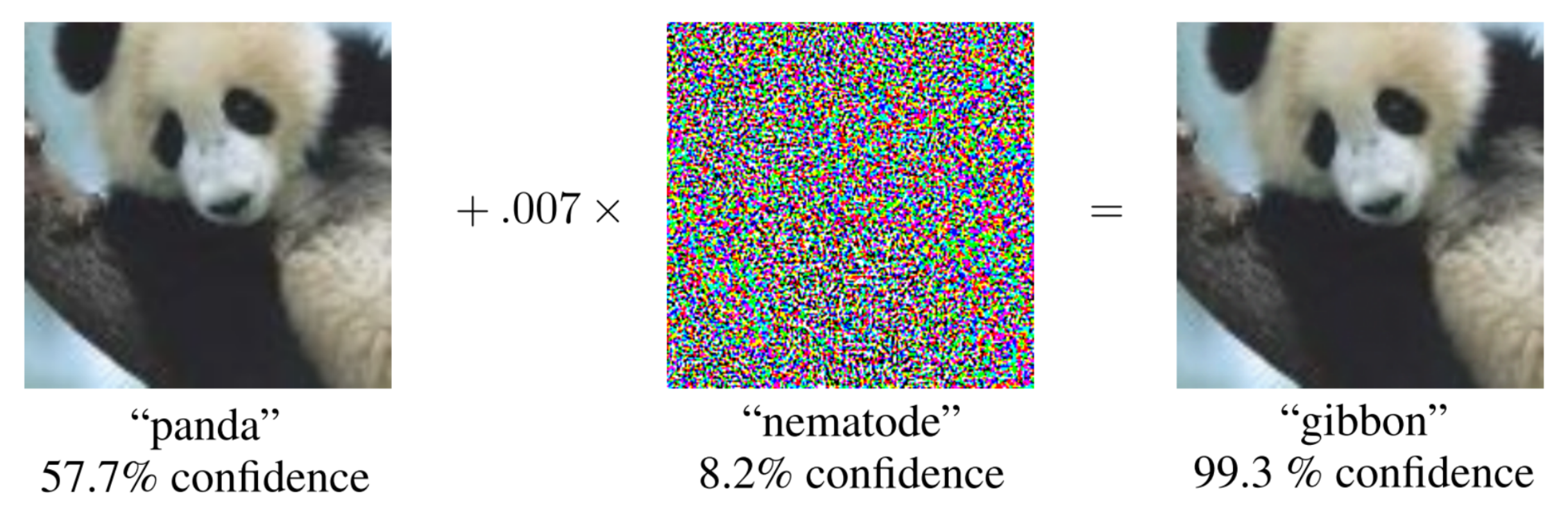
Not only is the difference between the left and right image imperceptable to humans, the classifier is also extremely certain in its ‘gibbon’ prediction. The existence of similar adversarial examples have also been found in many other contexts such as speech-to-text and reinforcement learning.
Naturally we want to prevent our models from being susceptible to these attacks so it is unsurprising that the discovery of adversarial examples has sparked a lot of research into robust neural networks. And with success! For example on the MNIST dataset (handwritten numbers) we can now train neural networks [2] that are guaranteed to be 87% accurate within a large radius: 40% change in each pixel’s brightness to be precise.
So we are done right? Well, not yet. While neural networks are good at working with unstructured data like images, audio and text, we often use different models for more structured data. Some of the best all-round models are … decision tree ensembles!
Decision trees and their ensembles
Decision trees are very simple models that consist of decision nodes whose decisions lead to a prediction leaf. Let’s look at an example.
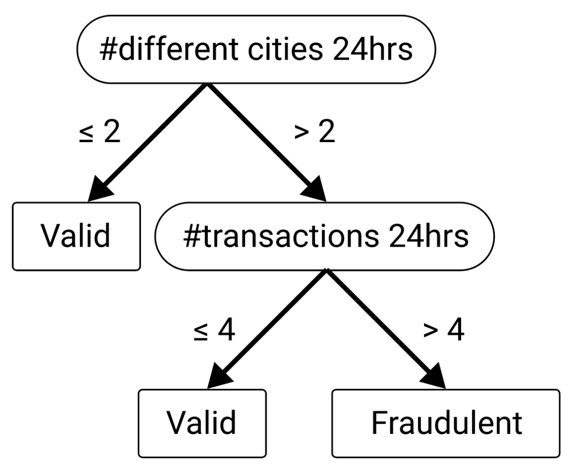
This decision tree was probably trained on a dataset of credit card transactions where the goal was to distinguish between valid and fraudulent transactions. The tree learned that by looking at just two features of the data (number of difference cities and transactions) it could predict fraudulent transactions decently well.
You can imagine that this tree is perhaps too simple and likely predicts a lot of false positives. It is therefore common to combine, tens, hundreds, or sometimes thousands of these trees in random forests or gradient boosting ensembles. These models are a top choice for predicting structured data.
But are these trees and ensembles robust?
Robustness of tree ensembles
To determine the robustness of decision trees and tree ensembles we want to know how often we can successfully create an adversarial example within some defined limits. In this blog post we will define these limits as a maximum L-infinity distance that an attacker can modify a sample by. In both the toy and MNIST examples we will limit the attacks within a distance of 10% of the feature range.
Now how do we find adversarial examples within these limits? In this blogpost we will use the MILP attack by [3]. This attack turns the model into a system of linear constraints (and binary variables) that an optimizer such as GUROBI can solve to find the optimal adversarial example. An optimal adversarial example is one with minimal distance from the original sample. Some adversarial examples generated using this attack are given in Figure 6.
Adversarial accuracy
A useful metric for determining robustness is the adversarial accuracy. It is the accuracy after an attacker has put in its best effort to attack each sample within the defined limits.
To compute this value we don’t have to solve an optimization problem to find the minimal adversarial example. Instead we just need to figure out whether any attack is possible within the limits and can do this by turning the standard MILP attack into a feasibility problem like the author of [4] did.
Decision regions of a toy dataset
Let’s look at some decision trees and ensembles trained on a 2D toy dataset, this way we can easily visualize the results. We create a toy dataset with a simple decision tree as the ground truth and take 100 samples from its space uniformly at random. For a random 10% of the samples we flip the labels to make the problem slightly harder:

Now let’s train a simple decision tree of depth 3, and a random forest on this dataset. We get the following scores on the train set and on a seperately generated test set:
| Model | Train accuracy | Test accuracy | Train adversarial accuracy | Test adversarial accuracy |
|---|---|---|---|---|
| Ground truth | 86% | 86% | 57% | 62% |
| Decision tree | 98% | 78% | 39% | 42% |
| Random forest | 100% | 78% | 17% | 19% |
The models score reasonably well on test accuracy but since they score much better on the training set there could be some overfitting. Aside from the overfitting problem there is also a large jump between regular accuracy scores and adversarial accuracy scores (about 40%-60% difference)! To see why this happens we visualize the decision spaces of the two models in Figure 4.


Two quick observations:
- There appear to be many small decision regions scattered throughout the space.
- The random forest predicts every training instance correctly.
To combat these two problems we will try the following:
- Increase the number of samples required for creating splits / leaves. Specifically, we allow the models to only create a leaf for 3 or more samples and only create decision nodes for 6 or more samples.
- Reduce the size of the forest’s bootstrap sample to 50% of the training set size so that the individual trees in the ensemble train on the same sample less often.
Now, we get the following scores:
| Model | Train accuracy | Test accuracy | Train adversarial accuracy | Test adversarial accuracy |
|---|---|---|---|---|
| Ground truth | 86% | 86% | 57% | 62% |
| Decision tree | 98% | 78% | 39% | 42% |
| Random forest | 100% | 78% | 17% | 19% |
| New decision tree | 87% | 80% | 47% | 49% |
| New random forest | 90% | 82% | 50% | 52% |
Clearly this has helped preventing the overfitting by reducing the train accuracy and increasing test accuracy. Even the adversarial accuracy scores went up. So how do the decision regions look?


While the regularized models look less chaotic, there are still unnecessary decision regions close to samples of opposite label. See for instance the red regions in the bottom-right corner of the random forest. Any sample close to that mix of colors can now easily become an adversarial example since there is always a blue/red region nearby to perturb to.
Clearly there are improvements left to make to get rid of the artifacts in the decision spaces. In a future blog post we will look at GROOT, a fast algorithm for fitting robust decision trees.
Beyond toy data: MNIST
Now that we have seen a small toy dataset and gotten some intuition on how decision tree models can be ‘fragile’ to adversarial examples, let’s look at some real data. We will test their performance on the MNIST handwritten digits dataset. We mentioned earlier that neural networks generally excel at predicting images while trees excel at predicting structured data. However, the MNIST dataset is relatively easy, so tree based models can still achieve good scores.
For this dataset we will set aside the single decision tree model as it is too simplistic for datasets with hundreds of important features (pixels). For simplicity, we will train a random forest only on two classes of the data: the model will try to distinguish between handwritten ‘2’s and ‘6’s. The forest contains 100 trees, only creates splits for 10 or more samples and only creates leaves for 5 or more samples.
| Model | Accuracy | Adversarial accuracy |
|---|---|---|
| Random forest | 99.7% | 16.0% |
After splitting in a 70%-30% train-test split the model predicts 99.7% of the test set correctly! Clearly this is a very good model, but is it robust? No. Given that an attacker can change each pixel’s brightness by 10% of the range, the attacker is successful in creating adversarial examples for 84% of the samples. That means the resulting adversarial accuracy is just 16%, worse than randomly guessing the label.
To get an idea of just how fragile the model is under adversarial influence we can look at some optimal adversarial examples. These are optimal in the sense that the L-infinity distance between the original sample and the misclassified adversarial example is minimal.


In summary
We briefly introduced decision trees, tree ensembles and how to attack these models with adversarial examples. We saw that on a small toy dataset the decision regions of these models look chaotic and might cause fragility to adversarial examples. Testing on a real dataset with handwritten digits we saw that a random forest was easily fooled by applying a tiny amount of noise onto the images.
In our research group we are interested in how to train trees and their ensembles to be robust against adversarial examples so please reach out with ideas / questions. In an upcoming blog post we will look at GROOT, an efficient algorithm for training robust decision trees.
References
[1] Goodfellow, Ian J., Jonathon Shlens, and Christian Szegedy. “Explaining and harnessing adversarial examples.” arXiv preprint arXiv:1412.6572 (2014).
[2] Zhang, Huan, et al. “Towards stable and efficient training of verifiably robust neural networks.” arXiv preprint arXiv:1906.06316 (2019).
[3] Kantchelian, Alex, J. Doug Tygar, and Anthony Joseph. “Evasion and hardening of tree ensemble classifiers.” International Conference on Machine Learning. PMLR, 2016.
[4] Andriushchenko, Maksym, and Matthias Hein. “Provably robust boosted decision stumps and trees against adversarial attacks.” arXiv preprint arXiv:1906.03526 (2019).